FinOps Inform

Save 20-50% on Spark Costs: Runbook Engineers Need

Engineers' runbook to cut Spark cloud spend 20-50%. Monitor job-level costs, triage top offenders, and apply stage-level sizing and external shuffle for measurable savings.

Kori September 10, 2026 · 10 min read

You can typically cut Spark cloud costs by 20 to 50% through three moves: instrument job-level cost attribution, right-size executors against actual stage demand, and offload shuffle to serverless or externalised storage where the workload pattern supports it. Public benchmarks show cost savings that depend heavily on how shuffle-heavy the workload is, ranging roughly from about a quarter to up to 85%. Measure first. The fixes below only work once you know which jobs are actually burning the budget.

TL;DR:

Tagging and ranking jobs by total and per-row costs enables targeted identification of the top 10 costliest Spark jobs for efficient optimization.

Enabling adaptive query execution and fixing scan volume or shuffle inefficiencies can reduce job costs significantly, especially in shuffle-heavy workloads.

Right-sizing executors with stage-level resource profiles offers potential savings of up to 50% by tailoring resources to specific stage demands.

Externalising shuffle storage can lower costs by up to 85% for shuffle-heavy queries, but only when combined with dynamic resource allocation and file compaction.

Conducting structured experiments with controlled configuration variations ensures sustained savings and avoids diminishing returns from ad hoc tuning.

Quick checklist: the 8 levers to try, first

Before touching a config file, get your triage list straight. This is the one-page runbook we hand to engineering teams on day one of a Spark cost optimization engagement.

Tag every job run with an identifier and join it against your cloud billing export.
Rank jobs by total cost and by cost-per-row, not just runtime.
Pull the top 10 cost offenders and open their Spark UI stage breakdown.
Check for partition pruning failures, tiny files, and unnecessary full scans.
Right-size executor cores and memory against actual peak stage usage.
Compact small files and standardise on a columnar format with sane row-group sizes.
Defer stage-level allocation, architecture rewrites, and re-platforming until you have baseline numbers.
Set auto-termination and minimum-size guardrails on any cluster you touch, even before deeper analysis.

That order matters. Riskier structural changes come later, once you have evidence rather than instinct guiding the decision.

How do you monitor and attribute Spark costs by job?

Cost attribution is the foundation of any Apache Spark cost reduction programme, and most teams skip it. Without a job-level cost figure, every optimisation conversation is a guess dressed up as an opinion.

Start by pulling the right billing signals. On EMR, that means instance-seconds and normalised units; on Glue, it means DPU hours surfaced through the GetJobRun and GetJobRuns APIs, joined with CloudWatch metrics. Neither of those numbers means anything until you attach them to a specific job run.

Ingest job-completion events (via EventBridge, job-run APIs, or scheduler webhooks) and compute cost per run in near real time.
Join billing data to job metadata: team, pipeline, environment, and business unit.
Build a leaderboard of highest-cost jobs, refreshed daily, not monthly.
Track cost-per-row or cost-per-record alongside raw job cost, since a job can get cheaper in total spend while getting worse per unit of work.
Alert on regressions: a sudden jump in cost-per-row, a new high-shuffle stage appearing after a code change, or p95 job cost drifting upward over a rolling week.

Pro Tip: Don't just alert on total spend. A job that doubles in data volume but keeps the same cost-per-row is healthy. A job with flat volume and rising cost-per-row is where your budget is quietly leaking.

Building this kind of dashboard from scratch is a genuine engineering project in its own right, and it's worth treating it as one rather than bolting cost metrics onto an existing observability stack as an afterthought, as we've covered in our guide to cloud observability for cost.

Why is this Spark job so expensive?

Once you know which jobs cost the most, the Spark UI and explain(cost) become your primary diagnostic tools. Open the stages tab first, not the SQL tab. Cost hides in stages, not in the logical query plan.

Four patterns account for the overwhelming majority of wasted spend:

Heavy shuffle: large shuffle read/write volumes relative to input size, usually from unnecessary wide transformations or poorly chosen join strategies.
Data skew: one or two tasks in a stage taking ten times longer than the median, dragging out the whole stage while most executors sit idle.
Small files: thousands of tiny partitions forcing excessive task scheduling overhead and wasted executor startup time.
Full table scans: missing partition pruning or predicate pushdown, meaning Spark reads far more data than the query logically needs.

Adaptive Query Execution addresses several of these automatically once enabled properly. Spark's own performance tuning documentation covers the specific settings, coalescing shuffle partitions, advisory partition sizing, and skew-join handling, that materially change shuffle behaviour without a line of application code changing.

The fastest way to validate a fix is a sampling replay: take a representative slice of production data, run the job locally or in a scratch cluster with the proposed configuration change, and compare stage-level metrics before and after. Don't push a config change straight to production and hope.

Pro Tip: If explain(cost) shows a broadcast join that isn't happening, check spark.sql.autoBroadcastJoinThreshold before you touch anything else. It's the single most common reason a join stage costs ten times what it should.

Fix scanned-data volume and shuffle volume first, in that order. Everything else, including executor sizing, matters less if the job is scanning three times more data than it needs to.

What are the best executor and cluster sizing settings?

Right-sizing is where most teams start, and where most teams stop too early, missing the deeper savings sitting in stage-level allocation.

A sensible starting point for executor sizing is a moderate number of cores per executor and a suitable amount of memory, adjusted for your specific workload's shuffle intensity and data skew profile. Wider executors beyond a certain size tend to have diminishing returns from garbage collection pressure and reduced parallelism per core; very narrow executors waste memory overhead per JVM.

Set spark.dynamicAllocation.enabled=true with sensible min/max executor bounds, not just a max.
Watch for the classic misconfiguration: dynamic allocation requesting executors aggressively at job start, then never releasing them because idle timeout is set too high.
Tune spark.dynamicAllocation.executorIdleTimeout down from the default if your jobs have bursty stage patterns.
Treat your first right-sizing pass as a baseline, not a final answer.

The deeper lever is stage-level allocation: instead of sizing the whole application uniformly, Spark's ResourceProfile API lets you size executors per stage. A shuffle-heavy stage might need wide, memory-rich executors; a simple filter stage further down the same job might run fine on a fraction of that footprint.

Research into stage-level executor allocation found cost savings of roughly 40 to 50% on benchmark queries, with slowdowns in the 16 to 29% range depending on the workload. That's a trade most cost-conscious teams will take gladly.

A reasonable experiment plan: pick two or three representative jobs, profile stage-level resource demand, apply differentiated ResourceProfile settings per stage, and measure cost and runtime against the uniform-executor baseline before rolling it out further.

Should you externalise Spark shuffle to cut costs?

Whether externalising shuffle helps depends entirely on your workload shape. Picture three patterns: an hourglass (heavy shuffle in the middle, light at the edges), an inverted triangle (shuffle-heavy throughout, tapering at the end), and a rectangle (steady, even resource demand start to finish). The first two benefit enormously from elastic, externalised shuffle; the rectangle usually doesn't, because there's no idle capacity to reclaim.

Enable serverless shuffle storage where your platform supports it, and pair it with dynamic resource allocation, since the two features compound.
Compact Parquet files regularly to avoid small-file overhead undermining any shuffle gains.
Co-locate storage and compute where latency-sensitive stages dominate runtime.

Benchmarking on EMR Serverless with serverless storage showed average cost reductions of around 26% across mixed queries, and up to 85% on shuffle-heavy queries with favourable shapes. Runtime can increase even as compute cost falls, so validate against your SLA before rolling it out broadly.

The caveat: externalised shuffle without dynamic resource allocation enabled delivers almost none of this benefit. The elasticity is the mechanism, not the storage tier itself.

When do spot instances and Graviton actually pay off?

Spot instances and ARM-based Graviton processors are two of the cheapest levers available, provided you cap the blast radius of interruptions.

Limit spot exposure per job rather than per cluster: a common pattern caps any single job at 30 to 50% spot executors, so an interruption event only affects a bounded fraction of running tasks.
On Kubernetes, pair a node provisioner such as Karpenter with a per-job spot balancer to hold that ratio automatically rather than relying on manual node-group configuration.
Validate Graviton compatibility on a representative job before committing: most pure Spark/JVM workloads run cleanly, but custom native libraries occasionally don't.
Run a small controlled test, same job, three instance-family variants, spot versus on-demand, before adopting either change fleet-wide.

Pro Tip: Graviton savings compound with spot savings. Test them separately first so you know which lever actually moved the number, rather than crediting both changes at once.

How do you run cost experiments and keep savings from eroding?

A structured experiment, sometimes called a FinHack, beats ad hoc tuning because it produces evidence rather than anecdote. One global financial services provider used exactly this approach, systematically testing instance types, spot mixes, and configuration changes, and cut EMR-related costs by roughly 30% over three months.

Select a representative sample of jobs, weighted toward your highest-cost offenders.
Vary one configuration dimension at a time, executor size, spot ratio, storage tier, and record cost, runtime, and failure rate for each variant.
Set governance guardrails alongside the experiments: mandatory tagging, auto-termination policies, and sensible minimum sizes for dev and staging clusters, none of which require code changes.
Feed results back into sprint planning, and consider tying a portion of an engineering team's targets to verified savings rather than raw feature velocity.

None of this needs to be elaborate. A shared spreadsheet tracking job, config variant, and measured outcome outperforms no experiment framework at all, every time.

What should engineers expect in the first 90 days?

Most teams underestimate how fast the first wins arrive, and overestimate how far generic tuning gets them. In the first 30 days, expect quick, low-risk wins: auto-termination policies, file compaction, and right-sizing executors on your top five cost offenders.

By 60 days, cost attribution dashboards should be live, giving you a defensible leaderboard rather than a hunch about what's expensive. By 90 days, deeper structural levers, stage-level allocation, spot and Graviton adoption, externalised shuffle, become viable because you now have baseline data to measure against.

We've seen this exact arc play out on other data platforms too. Our Snowflake cost optimization work followed the same measure-then-fix sequence, and the pattern holds regardless of which engine sits underneath your pipelines: attribution before optimisation, always.

Where Koritsu AI fits into your Spark cost reduction plan

If you've read this far, you already know the hard part isn't finding one setting to change, it's finding which of your dozens of Spark jobs are actually worth the engineering time. That's precisely the gap AI-driven cloud cost optimization solutions close. AI agents can continuously analyse cloud billing and job telemetry to surface which pipelines are burning budget, then engineering teams help fix the root cause rather than just resize a cluster and hope.

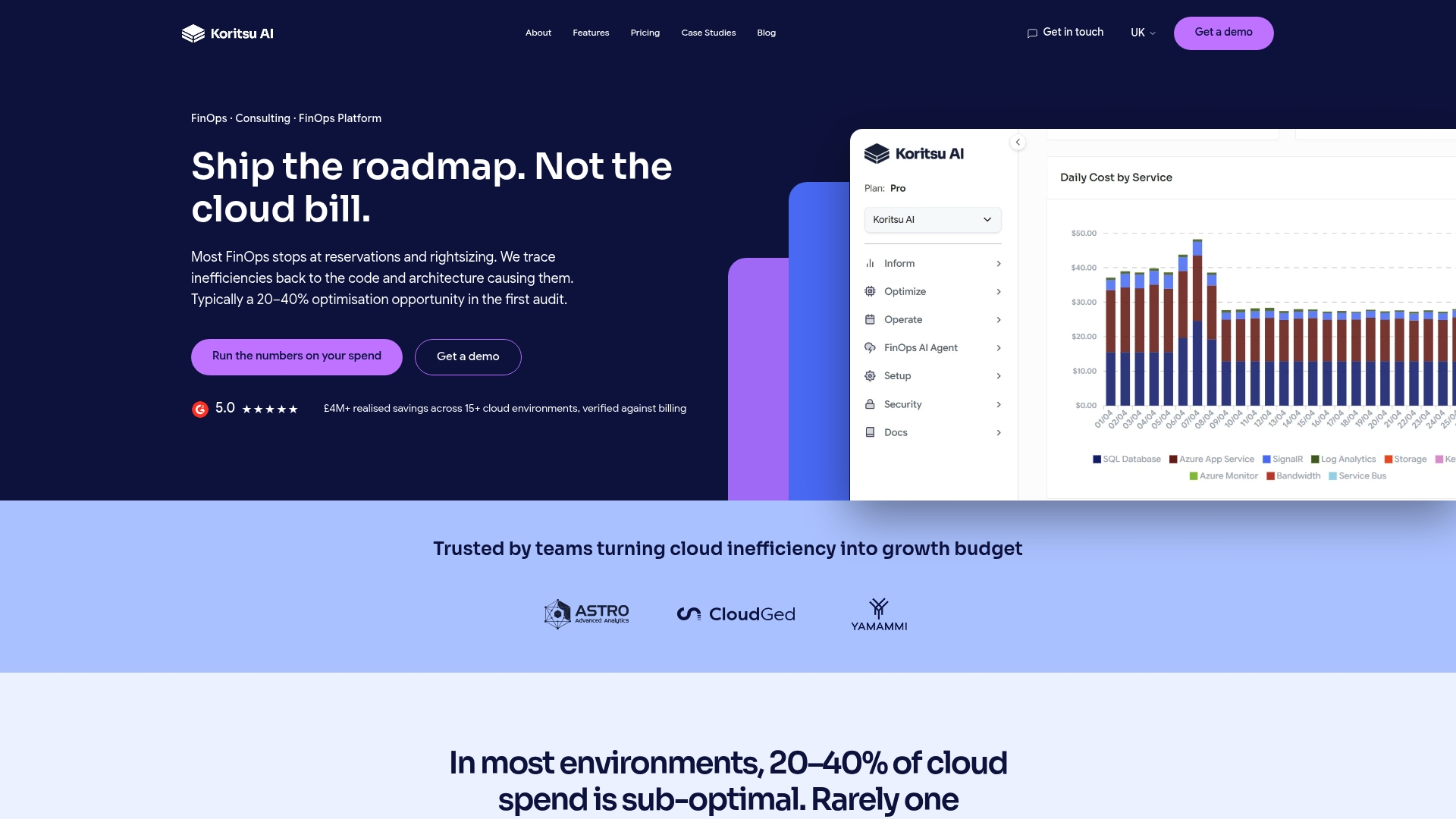
A free assessment shows you where the money is actually going before you commit to anything. From there, most engagements run on a success-fee basis, we take a share of verified savings, so the incentive is aligned with your outcome, not our billable hours. One UK bidding platform worked with us on exactly this model and cut cloud costs by 52% once the engineering fixes were identified and executed. If your Spark bill has been climbing without a clear explanation, starting with a cost assessment and AI analysis can reveal inefficiencies in your environment.

Sources

For teams building their own Spark cost optimization runbook, these are worth reading directly: Spark's own performance tuning documentation for AQE and shuffle settings, the IBM Research paper on stage-level allocation for the deeper cost-performance trade-off model, and AWS's Glue Flex jobs announcement for a concrete non-urgent-workload savings benchmark. On the broader cloud costing question, this comparison of Google Cloud pricing models is a useful companion read for teams weighing managed service costs beyond Spark alone.