BigQuery cost optimisation: a practical guide for engineers

The five actions below will cut your BigQuery bill within 72 hours. Apply them in this order: enforce explicit column selection in every query (immediate, high impact); set maximum_bytes_billed at the project or session level to cap runaway scans (immediate, high impact); enable default dataset and table expiration for all staging and transient tables (same day, medium impact), run dry runs before executing unfamiliar queries (immediate, low effort), and enable the BigQuery Recommenders alongside Cloud Billing export to BigQuery (within 24 hours, compounding impact over weeks).

• Immediate (today): Enforce column selection, set maximum_bytes_billed, run dry runs before any new query.
• Short (days): Enable billing export, turn on Recommenders, audit staging tables for missing expiration policies.
• Medium (weeks): Partition and cluster high-traffic tables, materialise repeated intermediate results.
• Long (months): Evaluate slot reservations once you have 30 days of utilisation data; consider autoscaling editions.

Those five actions address the most common sources of waste we see across UK engineering teams. The rest of this guide explains the mechanics behind each one, adds the architectural changes that compound savings over time, and shows how a real UK client verified the results.

---

Key takeaways

Fixing query hygiene before changing your pricing model is the single most reliable path to reducing BigQuery costs, because inefficient SQL wastes money regardless of whether you are on on-demand or slot-based pricing.

Point	Details
Enforce column selection	Replace SELECT * with explicit column lists to reduce scanned bytes on every query.
Set maximum_bytes_billed	Apply a hard byte cap at project or session level to prevent accidental large-scan charges.
Enable table expirations	Set default_table_expiration_ms on all staging datasets to stop silent storage accumulation.
Partition and cluster key tables	Apply the BigQuery Recommender's suggestions to tables with the highest bytes-scanned figures.
Koritsu AI free assessment	Koritsu AI delivers a prioritised savings report and implements fixes on a success-fee basis.

---

What does BigQuery actually charge you for?

BigQuery's pricing model splits into two independent dimensions: compute and storage. Most teams focus on one and ignore the other until the invoice arrives.

Compute: on-demand vs capacity

On-demand pricing charges per tebibyte (TiB) of data scanned by each query. You pay nothing when queries are idle, which makes it attractive for irregular workloads. Capacity pricing, sold as slot reservations under BigQuery Editions, charges per slot-hour regardless of whether those slots are busy. Slots are units of compute; a query that scans 10 TiB on a lightly loaded project may cost far less under capacity pricing if your team runs queries continuously throughout the day.

The crossover point depends on your query volume and concurrency. Teams with predictable, high-throughput workloads generally find capacity pricing more cost-effective once monthly spend on on-demand reaches a meaningful threshold. Teams with spiky or experimental workloads usually stay on on-demand longer.

Storage: active vs long-term

Storage is billed per byte per second. Two tiers apply: active storage (tables or partitions modified within the last 90 days) and long-term storage (untouched for 90 days or more). Long-term pricing reduces storage costs by about half once that threshold is reached, but deleting data or running time-travel queries can temporarily push partitions back into the active tier, which surprises teams expecting a clean discount.

You can also choose between logical billing (uncompressed bytes) and physical billing (compressed bytes on disk). Physical billing can be cheaper for highly compressible data, but it includes time-travel and fail-safe storage bytes, so the maths is not always straightforward.

Billing behaviours that catch teams out

Charged item	When it is incurred
Query bytes processed	At query execution; minimum 10 MiB per table referenced
Storage (active)	Per second, from table creation or last modification
Storage (long-term)	Per second, after 90 days without modification
Streaming inserts	Per row inserted via the streaming API
Batch loads (Cloud Storage)	Free for load jobs from Cloud Storage
Slot reservations	Per slot-hour, regardless of utilisation

The 10 MiB minimum per table referenced is one of the most overlooked billing behaviours. A query that joins five small lookup tables will be billed as if each one contained at least 10 MiB of data. For teams running thousands of micro-queries against small dimension tables, this adds up quickly. BigQuery also offers a free tier covering the first 1 TiB of query data processed per month per project, which is useful for development environments but rarely meaningful for production workloads.

---

How to cut BigQuery storage costs before they compound

Storage costs grow silently. A pipeline that writes a staging table daily without an expiration policy will accumulate months of data that nobody queries. The fix is architectural, not reactive.

Set default table and dataset expirations

Apply a default table expiration to every dataset that holds transient or staging data. In the BigQuery console or via Terraform, set default_table_expiration_ms at the dataset level. Tables created within that dataset inherit the expiration automatically, so new pipelines cannot accidentally accumulate indefinitely. For datasets that mix permanent and transient tables, set expiration at the table level during creation rather than relying on the dataset default.

Implement expirations safely by first auditing which tables are actively queried using INFORMATION_SCHEMA.TABLE_METADATA_TIMELINE or the billing export. Tables with zero query activity in the past 30 days are candidates for expiration or archival.

Use long-term storage deliberately

Partition tables by date or timestamp columns. Partitions that are not modified for 90 days automatically transition to long-term pricing, reducing storage costs by about half for that partition. The key is to avoid unnecessary writes: a pipeline that rewrites an entire historical partition to fix a single row will reset the 90-day clock on that partition and push it back to active pricing.

When you do need to delete data, prefer partition-level DELETE or DROP PARTITION operations over full table rewrites. Time-travel retention (7 days by default) means deleted data still incurs storage charges for a short window, so factor that into cost projections.

Avoid duplicate copies with federated and external tables

Teams often copy data into BigQuery from Cloud Storage or other sources when a federated query would suffice. External tables let you query data stored in Cloud Storage, Google Drive, or Cloud Bigtable without loading it into BigQuery storage. The trade-off is query performance: external queries do not benefit from BigQuery's columnar storage or caching. Use external tables for infrequently queried reference data or archival datasets where query latency is acceptable.

Streaming inserts vs batch loads

Streaming inserts via the BigQuery Storage Write API or the legacy streaming API incur a per-row charge. Batch loads from Cloud Storage are free. If your pipeline can tolerate a delay of minutes rather than seconds, switching from streaming to micro-batch loads is one of the fastest ways to reduce ingestion costs. Review every pipeline that uses streaming and ask whether the latency requirement genuinely justifies the cost.

Pro Tip: Set default_table_expiration_ms on every staging dataset as part of your infrastructure-as-code template. A dataset created without an expiration policy is a future storage bill waiting to happen.

---

Query hygiene: the fastest way to reduce on-demand charges

Query costs on on-demand pricing are determined entirely by bytes scanned. Every byte you avoid scanning is money saved. The best practices documentation is clear on this: fix the SQL before you touch the pricing model.

Stop scanning columns you do not need

SELECT * is the single most expensive habit in BigQuery. Because BigQuery uses columnar storage, selecting only the columns your query needs can reduce scanned bytes dramatically.

-- Expensive: scans all columns
SELECT * FROM `project.dataset.events` WHERE event_date = '2025-01-01';

-- Cheaper: scans only what you need
SELECT user_id, event_type, revenue
FROM `project.dataset.events`
WHERE event_date = '2025-01-01';

LIMIT does not reduce bytes scanned on non-clustered tables. This surprises many engineers who assume it works like a database cursor. BigQuery scans the full column data before applying the limit, so SELECT * FROM large_table LIMIT 10 is just as expensive as SELECT * FROM large_table.

Dry runs and the query validator

Before executing any unfamiliar or large query, use a dry run to estimate bytes scanned without incurring a charge. In the console, the query validator shows the estimated bytes in the bottom-right corner. Via the API or bq CLI, pass --dry_run to get the byte estimate programmatically.

bq query --dry_run --use_legacy_sql=false \
  'SELECT user_id FROM `project.dataset.events` WHERE event_date = "2025-01-01"'

Build dry runs into your CI/CD pipeline for any query that will run in production. A query that scans 500 GiB on every execution is a governance failure, not a one-off mistake.

Set maximum_bytes_billed as a hard cap

maximum_bytes_billed is a session-level or query-level parameter that causes BigQuery to reject any query exceeding the specified byte threshold. Set it at the project level via a default value in your connection configuration, and override it only for queries that genuinely need a higher limit.

from google.cloud import bigquery

client = bigquery.Client()
job_config = bigquery.QueryJobConfig(
    maximum_bytes_billed=10 * 1024**3  # 10 GiB cap
)

This is not a performance optimisation. It is a governance control. A developer who accidentally runs a full-table scan on a 50 TiB dataset will get an error rather than a surprise invoice.

Materialise intermediate results

Queries that reference the same large intermediate result multiple times should write that result to a destination table or use a materialised view. BigQuery does not cache intermediate results across query steps by default, so a complex pipeline that re-derives the same aggregation in three downstream queries will scan the source data three times.

Materialised views refresh automatically on a schedule and serve cached results when the underlying data has not changed, making them particularly useful for dashboards and recurring reports. For one-off pipelines, writing to a destination table and querying that table downstream achieves the same effect.

Approximate aggregations and reducing shuffles

For analytics that do not require exact counts, APPROX_COUNT_DISTINCT uses the HyperLogLog++ algorithm and is significantly faster and cheaper than COUNT(DISTINCT ...) on large datasets. Similarly, APPROX_QUANTILES and APPROX_TOP_COUNT reduce the data shuffled across slots.

Heavy JOIN operations and window functions with large PARTITION BY clauses are the most common sources of slot waste. Profile expensive queries using the query execution plan in the console (the "Execution details" tab) to identify stages with disproportionate shuffle or input bytes.

Pro Tip: Add a maximum_bytes_billed check to your code review checklist for any query that will run on a schedule. If a reviewer cannot estimate the byte cost of a new query, it should not merge without a dry run result attached.

---

How partitioning and clustering reduce scanned bytes

Partitioning and clustering are the two structural changes that have the highest long-term impact on BigQuery cost optimisation. Both work by allowing BigQuery to skip blocks of data that cannot match a query's filter conditions.

Partitioning: prune entire partitions

A partitioned table divides data into segments based on a date, timestamp, or integer column. When a query includes a filter on the partition column, BigQuery reads only the relevant partitions rather than the full table.

-- Without partitioning: scans entire table
SELECT * FROM events WHERE DATE(created_at) = '2025-06-01';

-- With date partitioning on created_at: scans only the 2025-06-01 partition
SELECT user_id, event_type FROM events WHERE DATE(created_at) = '2025-06-01';

Ingestion-time partitioning (_PARTITIONTIME) is the simplest option for append-only pipelines. For tables with a meaningful business timestamp, partition on that column instead. Avoid over-partitioning: tables with millions of tiny partitions (under 1 GB each) incur metadata overhead and can slow query planning.

Clustering: prune blocks within partitions

Clustering sorts data within each partition by up to four columns, allowing BigQuery to skip entire storage blocks when a query filters on those columns. Clustering is most effective on high-cardinality columns that appear frequently in WHERE clauses or JOIN conditions: user_id, product_id, region.

Combining partitioning and clustering is the standard pattern for large tables. Partition by date, cluster by the most selective filter column. The block-pruning benefit from clustering compounds with partition pruning, so a query that filters on both the partition column and a cluster column can scan a small fraction of the total table.

Common mistakes to avoid

• Partitioning on a column with very low cardinality (e.g. a boolean flag) creates few large partitions and provides minimal pruning benefit.
• Clustering on columns that never appear in query filters adds write overhead with no read benefit.
• Creating excessive small partitions (daily partitions on a table that receives only a few rows per day) inflates metadata costs and slows partition management operations.
• Forgetting to include the partition column in WHERE clauses, which forces a full-table scan despite the partition structure.

Using the Recommender to guide decisions

The BigQuery partitioning and clustering recommender analyses up to 30 days of workload execution data and returns specific column recommendations with estimated monthly savings. It is the most reliable starting point because it uses your actual query patterns rather than assumptions.

One caveat: the recommender can overestimate savings for multi-stage queries that reference the same table multiple times across pipeline steps. Treat its estimates as directional rather than precise, and verify savings against actual bytes billed after applying a recommendation.

Pro Tip: Check the Recommender output in the BigQuery console under "Recommendations" before manually designing a partition scheme. It will often surface a column you had not considered, backed by 30 days of real workload data.

---

When should you consider slot reservations?

On-demand pricing is the right default. Slot reservations make sense only when your workload meets specific conditions, and committing too early is a common and expensive mistake.

Decision checklist for moving to capacity pricing

1. Your monthly on-demand spend has been consistent for at least 60 days with low variance.
2. You have identified the peak concurrent slot demand using INFORMATION_SCHEMA.JOBS_BY_PROJECT and it is predictable.
3. You have exhausted query hygiene improvements (column selection, partitioning, clustering, materialisation) and the remaining spend is structural, not behavioural.
4. You have modelled the slot-hour cost against your current on-demand spend and confirmed a saving at your actual utilisation rate.

If you cannot tick all four, stay on on-demand and fix the inefficiencies first.

How to estimate your slot needs

Query INFORMATION_SCHEMA.JOBS_BY_PROJECT to extract total_slot_ms per job over the past 30 days. Divide by the total milliseconds in that period to get average slot utilisation, and look at the 95th percentile for peak demand. The BigQuery slot estimator in the console provides a similar view without writing SQL.

SELECT
  TIMESTAMP_TRUNC(creation_time, HOUR) AS hour,
  SUM(total_slot_ms) / (1000 * 3600) AS avg_slots
FROM `region-eu.INFORMATION_SCHEMA.JOBS_BY_PROJECT`
WHERE creation_time BETWEEN TIMESTAMP_SUB(CURRENT_TIMESTAMP(), INTERVAL 30 DAY)
  AND CURRENT_TIMESTAMP()
GROUP BY 1
ORDER BY 1;

Autoscaling and commitment trade-offs

BigQuery Editions (Enterprise and Enterprise Plus) include autoscaling, which allows slot capacity to scale up and down per second based on demand. This is billed per slot-second, so you pay only for what you use above your baseline reservation. For workloads with significant peaks, autoscaling with a modest baseline reservation often costs less than a large fixed commitment.

One-year commitments offer a discount over monthly rates; three-year commitments offer a larger discount but lock in capacity for a long period. Google Cloud's guidance is consistent: start with monthly or short-term reservations, monitor utilisation for at least 30 days, and only then consider annual commitments.

Governance patterns for reservations

• Assign reservations to specific projects or folders using reservation assignments to prevent one team's heavy workload from consuming capacity allocated to another.
• Enable idle-slot sharing so that unused slots in one reservation can be borrowed by other assignments, improving overall utilisation.
• Set per-project and per-user daily query quotas via the Cloud Billing controls to prevent a single runaway job from exhausting shared capacity.

---

How to make BigQuery cost control continuous

Manual optimisation degrades over time. New tables get created without expiration policies. New queries bypass column selection. A governance model that relies on periodic audits will always lag behind the bill. The solution is to instrument your environment so that anomalies surface automatically.

Enable Cloud Billing export and job metadata

1. Enable Cloud Billing export to BigQuery from the Google Cloud Console under Billing > Billing export. Select the BigQuery dataset where export data will land.
2. Export job metadata by enabling INFORMATION_SCHEMA access for your region. Key fields: total_bytes_billed, total_slot_ms, user_email, referenced_tables.
3. Retain at least 90 days of billing export data to support trend analysis and anomaly detection.
4. Build a cost-by-user or cost-by-dataset report using the exported data.

-- Cost by user (last 30 days, on-demand pricing at $6.25/TiB)
SELECT
  user_email,
  SUM(total_bytes_billed) / POW(1024, 4) AS tib_billed,
  ROUND(SUM(total_bytes_billed) / POW(1024, 4) * 6.25, 2) AS estimated_cost_usd
FROM `region-eu.INFORMATION_SCHEMA.JOBS_BY_PROJECT`
WHERE creation_time >= TIMESTAMP_SUB(CURRENT_TIMESTAMP(), INTERVAL 30 DAY)
GROUP BY 1
ORDER BY 3 DESC;

This query surfaces which users or service accounts are driving the most spend, which is the starting point for targeted governance conversations. For building a full internal cost dashboard from this data, the Koritsu FinOps dashboard guide covers the architecture in detail.

Turn on Recommenders

• Navigate to BigQuery > Recommendations in the Google Cloud Console.
• Enable the Partitioning Recommender, Clustering Recommender, and Slot Recommender for each project.
• Review recommendations weekly. Each recommendation includes an estimated saving and the workload evidence behind it.
• Use INFORMATION_SCHEMA.RECOMMENDATIONS to query recommendations programmatically and integrate them into your FinOps reporting.

Budgets, alerts and anomaly detection

Alerts fire via email or Pub/Sub, which allows automated responses (for example, disabling a service account that has exceeded its quota). For cloud observability patterns that extend beyond BigQuery, the same alerting architecture applies across GCP services.

---

How to prioritise fixes and what verified savings look like

The most common mistake in BigQuery cost reduction is starting with the most technically interesting change rather than the highest-impact one. Reservations are intellectually engaging. Fixing SELECT * in 40 production queries is tedious. The tedious fix usually saves more money.

Prioritisation framework

• Quick wins (this week): Set maximum_bytes_billed, enforce column selection in the top 10 most expensive queries (by total_bytes_billed), add expiration policies to all staging datasets.
• High ROI (next 2–4 weeks): Apply partitioning and clustering to the top 5 tables by bytes scanned, materialise the most frequently re-derived intermediate results.
• Platform changes (next 1–3 months): Evaluate slot reservations with 30 days of utilisation data, configure autoscaling, implement reservation assignments.

Measure the baseline before making any change. Record total_bytes_billed and total_slot_ms per day for the two weeks before a change, then compare against the two weeks after. Invoice reconciliation confirms that estimated savings translate to actual billing reductions.

Koritsu AI case study: UK bidding platform

A UK-based bidding platform came to Koritsu AI with a BigQuery bill that had grown significantly quarter-on-quarter despite no major increase in data volume. The root causes were a combination of missing partition filters in production queries, staging tables accumulating months of data without expiration policies, and a slot reservation sized for peak load that ran at low utilisation most of the time.

Koritsu AI's assessment identified that the platform's top 15 queries by bytes billed were all missing partition filter predicates, meaning every query performed a full-table scan on tables that were already partitioned. Adding the missing WHERE clause on the partition column to each query, combined with setting expiration policies on staging datasets and right-sizing the slot reservation, produced a 52% reduction in cloud costs verified against three consecutive monthly invoices.

The verification approach used a time-window comparison: baseline spend from the three months before remediation versus the three months after, controlling for data volume growth. The saving was confirmed in the billing export, not estimated from dry runs.

Pro Tip: Train developers to attach a dry run byte estimate to every pull request that introduces a new scheduled query. This single behavioural change, enforced at code review, prevents expensive queries from reaching production without scrutiny. The developer choices guide covers the broader cultural patterns that compound these savings.

---

The traps UK engineering teams keep falling into

Most BigQuery cost problems are not technical failures. They are process failures dressed up as technical ones.

The most persistent trap we see is teams that provision slot reservations to "solve" a cost problem without first addressing the queries driving that cost. A reservation does not make an inefficient query cheaper; it just changes who pays for the inefficiency. If your top 20 queries each scan 10 TiB because nobody enforces column selection, buying slots shifts the billing model but does not reduce the underlying waste. Fix the queries first. The reservation decision becomes straightforward once the workload is clean.

The second trap is micro-query proliferation. Teams building event-driven pipelines or real-time dashboards sometimes fire hundreds of small queries per minute against dimension tables. Each query hits the 10 MiB minimum per table referenced, so a query that scans 50 KB of actual data is billed as 10 MiB. At scale, this is a significant hidden cost. The fix is to cache dimension data in application memory or use materialised views rather than querying BigQuery for every event.

The cultural fix for both traps is the same: make cost visible at the point where decisions are made. A FinOps ritual as simple as a weekly 15-minute review of the top 10 queries by bytes billed, shared with the engineering team, changes behaviour faster than any governance policy. Pair it with a code review gate that requires a dry run estimate for any new scheduled query, and you have a lightweight process that compounds savings over time. The cloud deployment cost checklist provides a broader framework for embedding these controls into your engineering workflow.

---

What Koritsu AI does when you need hands-on help

Most teams know what they should do. The gap is between knowing and doing it systematically, with verified results.

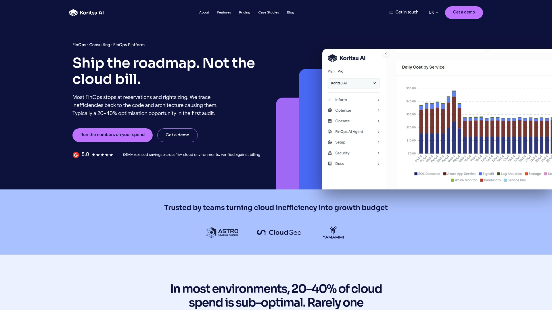
Koritsu AI's engagement starts with a free assessment of your BigQuery environment: we analyse your billing export, query patterns, and storage configuration to produce a prioritised savings report. From there, our specialists work alongside your engineering team to implement the fixes, not just recommend them. Our AI agent, Kori, monitors your environment continuously and surfaces new anomalies as your workload evolves.

The UK bidding platform case study shows what a verified engagement looks like: a 52% cost reduction confirmed against three months of invoices, not estimated from a spreadsheet. We charge on results, taking a share of the savings we actually deliver. There is no upfront fee and no long-term contract to sign before you see value. If you want to know what your BigQuery environment is wasting, start with the free assessment.

---

Sources

The links below are the primary references for implementing and verifying the steps in this guide.

• BigQuery pricing
• This page describes best practices for estimating and controlling costs in BigQuery.

Recommended

• Benefits of cloud observability for cost: 2026 guide | Koritsu Blog
• What is cloud cost optimisation? 2026 guide | Koritsu Blog
• How to reduce cloud infrastructure costs in 2026 | Koritsu Blog
• How to optimise API calls in cloud services | Koritsu Blog